Detecting nearly duplicate images using wavelet transforms

n.b. This is a very early draft of this post, expect typos, grammatical errors, factual inaccuracies, etc.

One of the first things that became obvious while working on Vignette was the need to identify and group nearly duplicate images. Like myself, the friend who donated his photos to this project frequently takes multiple photos of the same scene in quick succession. This is a smart strategy – storage is cheap and it hedges against focus issues, exposure problems, and motion blur. However, it can make browsing through photos somewhat tedious, and more importantly, can make it easier to lose sight of the larger “picture” while looking back on a day or experience.

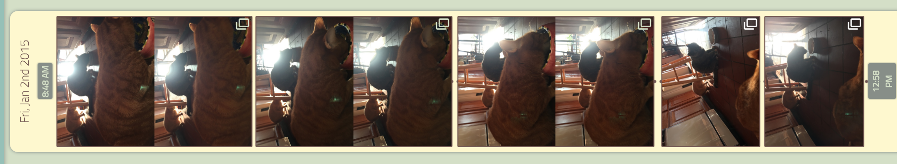
Note, critically, that these duplicate images are not exactly the same – there are minor differences in framing/orientation, in exposure, and in white balance. Therefore, we call these images “near duplicates.” Identifying and grouping these near duplicate images is a non-trivial task.

The naive approach: direct comparison

A naive approach for comparing near duplicate images might be to look at the pixel values directly. For example, we could calculate the Euclidean distance between two images. (sqrt(sum((A-B)^2)), where A and B are image vectors.) However, this does not work very well.

A small variation in exposure produces an offset with every pixel value, which can make very similar images seem very far from each other. A small change in perspective or a small rotation can likewise produce a very large Euclidean distance.

Finally, noise is a significant issue – even if the image was taken using a tripod, minor value variation caused by noise will accumulate across the entire image.

Histogram comparison

There are various references in literature to finding near duplicate images through the comparison of image histograms, however, I did not have success with this method.

Todo: explain?

Wavelet transform

Wavelet transforms are frequently used for image compression and analysis. This is because wavelets have several important advantages over other representation bases. One of these advantages is “sparsity.”

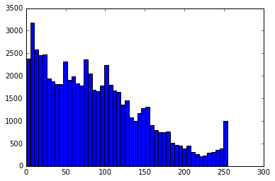
We can see this by looking at the distribution of values in a wavelet transformed image vs. the original image pixel values. A histogram of the pixel values of the original image shows a roughly uniform distribution – i.e., a pixel is as likely to have a value of 0, as it is of 100, or 255.

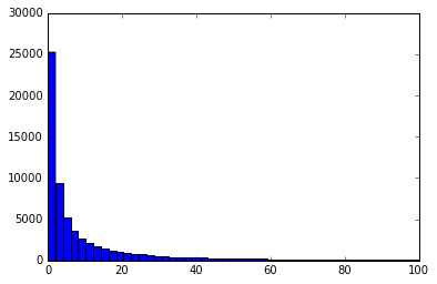
The histogram of the image after a wavelet decomposition is very different – the vast majority of the values in the transformed version are close to 0, and larger values are exponentially less likely.

This means that many values can be truncated to 0, allowing wavelet transforms to preserve details much better than by simply downsampling the image, as the comparison below shows. The left-hand column shows a simple downscaling/pixellation, and the right-hand column shows an image formed from a inverting a sparse-ified wavelet decomposition. Click on the image for a full resolution comparison. Note how the inverted wavelet transform image has preserved detail in regions where there are fine and dramatic brightness variations.

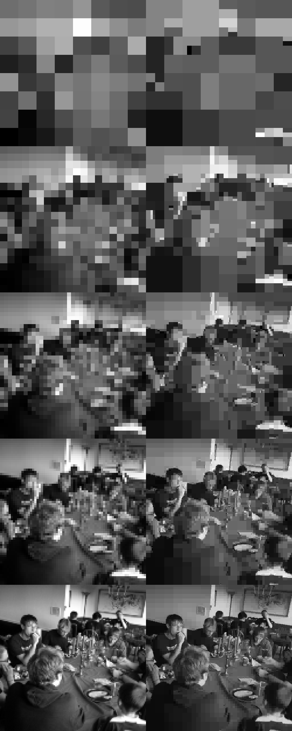
Each image in the comparison, whether a simple downsampled image or a sparsely sampled wavelet transformed image has roughly the same number of bytes. Note how the wavelet decomposed images preserve more perceptual detail.

This small, sparse wavelet transform can be viewed as a kind of “syntactic fingerprint” of the image. “Syntactic” because it describes literally what an image looks like, and not what it represents (a “semantic” fingerprint, which we will discuss later.)

Types of wavelet transforms

Wavelet decompositions come in many flavors, based on the “wavelet” that is used. The simplest, and what we will use in this article, is the Haar wavelet, which simply looks like a square, or a primitive highpass filter, computing sequential differences.

Decomposing a 1-D sequence, such as [8, 9, 9, 12, 3, 1, 5, 6] with the Haar wavelet involves convolving the sequence with a scaled and stretched version of this wavelet – esentially a series of differences.

The first level of decomposition might look like [8.5, 10.5, 2, 5.5, 0.5, 1.5, -1, 0.5]. Note how the first four values in the sequence are the average of two sequential terms in the original series, and the second four values encode the differences between two sequential terms. So, the first value in the original series, 7, is equal to 7.5 - 0.5.

Now, the first four elements in the decomposition can be decomposed again. (Because each value here spans two original values, we now have a stretched wavelet.) This results in: [9.5, 3.75, 1, 1.75, 0.5, 1.5, -1, 0.5]. We can perform the decomposition one time further, to find the final, multi-level Haar wavelet decomposition: [6.625, -2.875, 1, 1.75, 0.5, 1.5, -1, 0.5]. Note that the majority of the values are very close to 0!

By eliminating all values below some threshold (let’s say 1), we can create a sparse vector: [6.625, -2.875, 0, 1.75, 0, 1.5, 0, 0]. Reconstructing the full sequence from this sparse vector results in the following:

[6.625, -2.875, 0, 1.75, 0, 1.5, 0,   0]
[9.5,   3.75,   0, 1.75, 0, 1.5, 0,   0]
[9.5,   9.5,    2, 5.5,  0, 1.5, 0,   0]
[9.5,   9.5,    8, 11,   2, 2,   5.5, 5.5]

While the values are not exact, the “shape” of the sequence is approximately preserved, with only four values! (Of course, you also need to store the position of those four values.)

Haar wavelets are only one form of wavelet decomposition. There are other varieties of wavelet bases, including the Mexican hat:

and the somewhat unexpected looking 4-tap Daubechies wavelet:

Decomposing an image

It is straightforward to decompose an image using the PyWavelets python library. The only annoying part is converting the tuple format that PyWavelets uses into a singla array. (Done here with pack_wavelet_coeffs.)

def get_luminance(im):
	im = np.asarray(im.copy(), dtype=np.float32)
	im = 0.25 * (im[:,:,0] + 2 * im[:,:,1] + im[:,:,2])
	return im

def get_square_crop(im):
	transposed = False
	
	if im.shape[1] > im.shape[0]:
		im = np.transpose(im)
		transposed = True
	
	im = im[((im.shape[0] - im.shape[1])/2):((im.shape[0] + im.shape[1])/2),:]
	
	if transposed:
		im = np.transpose(im)
		
	return im

def antialiased_imresize(im, new_size):
	r = float(new_size[0]) / im.shape[0]
	im = filters.gaussian_filter(im, [0.25/r, 0.25/r])
	im = scipy.misc.imresize(im, r, interp='nearest')
	return im

def pack_wavelet_coeffs(w, level=4):
	pw = np.zeros(2**((level-1)*2), dtype=np.float32)

	pw[0:len(np.ravel(w[0]))] = np.ravel(w[0])
	ni = len(np.ravel(w[0]))

	for i in range(1,level):
		for j in range(0,3):
			pw[ni:ni+len(np.ravel(w[i][j]))] = np.ravel(w[i][j])
			ni += len(np.ravel(w[i][j]))
	return pw

def get_sparse_haar_coefficients(im, ncoeffs = 40, level=4):
	w = pywt.wavedec2(im, 'Haar')
	pw = pack_wavelet_coeffs(w, level=level)

	# set all except the maximum ncoeffs coefficients to 0
	maxi = np.argsort(np.abs(pw))
	pw[maxi[:-ncoeffs]] = 0

	# normalize coefficients
	pw = pw / np.sqrt(np.sum(pw**2))
	
	return pw

def get_fingerprint(im, ncoeffs=40, level=4):
	# crop and scale each image to a consistent size
	im = get_square_crop(get_luminance(im))
	im = antialiased_imresize(im, [1024.001, 1024.001]) 

	# return the syntactic fingerprint  
	pw = get_sparse_haar_coefficients(im, ncoeffs=ncoeffs, level=level)
	return pw

Finding near duplicate images using sparse wavelet comparisons

Remember that the issues we faced with Euclidean distance for image comparison were primarily image noise, changing image viewpoints, and changing exposure/white balance.

Removing small values from the wavelet decomposition proves not only to be effective at compressing the amount of information that we need to share, it also smooths out minor variations due to noise, while still preserving sharp edges and major variations. This means that a Euclidean comparison on the sparse wavelet vectors much more resistant to image noise. (This is also why wavelet transforms are so frequently used for image de-noising!)

How does it help with shifting image perspective though? We’re still preserving all of the details in the same spot, so it initially seems like it wouldn’t help at all. Indeed, this is where this method struggles the most – still, we can build some robustness to small variations in image angle by limiting the maximum resolution of the reconstruction. The shift of a downscaled image is similarly downscaled.

Finally, to compensate for differences in exposure or white balance, we simply normalize the wavelet transfomed values. Todo: this does seem to work better than normalizing just the original image, but why would this be?

def get_fingerprint_difference(im1, im2, debug=False, level=4):    
	pw1 = get_fingerprint(im1, level=level)
	pw2 = get_fingerprint(im2, level=level)
	
	fingerprint_difference = (np.sqrt(np.sum(np.power(pw1 - pw2, 2))))
	
	return fingerprint_difference

Extra information: timestamps

The timestamp associated with each image also provides an important clue. Without knowing anything at all about image content, images taken one second apart are certainly more likely to be duplicates than those taken one minute apart. We can incorporate this into our final model.

The final duplicate detection model

Using a small, manually tagged dataset, a logistic regression was performed on two input variables, the time difference and the Euclidean difference between the sparse wavelet decompositions.

def probability_of_duplicate(fingerprint_similarity, time_delay):
	# magic numbers are a logistic regression to the training set
	p = np.exp(-3.5423 + 13.7986 * fingerprint_similarity + 0.1512 * time_delay) / (1 + np.exp(-3.5423 + 13.7986 * fingerprint_similarity + 0.1512 * time_delay))
	return (1 - p)

Todo: expand this section with more details. Make a more formalized training process for this.

A better approach: image features

However, this wavelet-based near duplicate image detector still has plenty of room for improvement. Notice that the near duplicate images used as an example at the beginning of the article are actually arranged in several distinct groups.

This is because the wavelet-based near duplicate image detector does not recognize the ungrouped images as duplicates. Yet, it is not difficult to argue that at least some of them ought to be considered duplicates of each other.

A better method for detecting near-duplicates might be using a feature detector to compare common features between images, and then test for spatial consistency of those features. We will do this next week, using SURF, FLANN, and RANSAC.